Recommendation System Evaluation

2023-10-03
ML Applications

Evaluation Metrics in Recommendation System

Accuracy and Error Based Metrics

Mean Absolute Error (MAE)

Given a movie rating dataset[2], it calculates the average absolute difference between predicted and actual ratings.

1
2
3
4
5
6
7
8
9
10
11
12
13
14
15
16
17
18
19
20
21
22
23
def mean_absolute_error(actual_ratings, predicted_ratings):
# Check if the lengths of actual_ratings and predicted_ratings are equal
if len(actual_ratings) != len(predicted_ratings):
raise ValueError("The length of actual_ratings and predicted_ratings must be the same.")

n = len(actual_ratings)
total_error = 0

# Iterate through the lists and calculate the absolute difference between actual and predicted ratings
for i in range(n):
total_error += abs(actual_ratings[i] - predicted_ratings[i])

# Calculate the average of absolute differences
mae = total_error / n
return mae

# Example usage
actual_ratings = [3.5, 4.0, 2.0, 5.0, 3.0]
predicted_ratings = [3.0, 4.5, 1.5, 4.5, 2.5]

# Call the mean_absolute_error function with actual_ratings and predicted_ratings
mae = mean_absolute_error(actual_ratings, predicted_ratings)
print(f"Mean Absolute Error: {mae}") # 0.5

Root Mean Square Error (RMSE)

Mean Square Error (MSE) calculates the average squared differences between predicted and actual ratings, which helps to negate the negative sign but it scales up the errors that cannot be compared to actual rating values due to different rating scales.

In RMSE, it takes the square root of MSE to normalize the scale issue that MSE had.

1
2
3
4
5
6
7
8
9
10
11
12
13
14
15
16
17
18
19
20
21
22
23
24
25
import math

def root_mean_square_error(actual_ratings, predicted_ratings):
# Check if the lengths of actual_ratings and predicted_ratings are equal
if len(actual_ratings) != len(predicted_ratings):
raise ValueError("The length of actual_ratings and predicted_ratings must be the same.")

n = len(actual_ratings)
total_error = 0

# Iterate through the lists and calculate the squared difference between actual and predicted ratings
for i in range(n):
total_error += (actual_ratings[i] - predicted_ratings[i]) ** 2

# Calculate the square root of the average of squared differences
rmse = math.sqrt(total_error / n)
return rmse

# Example usage
actual_ratings = [3.5, 4.0, 2.0, 5.0, 3.0]
predicted_ratings = [3.0, 4.5, 1.5, 4.5, 2.5]

# Call the root_mean_square_error function with actual_ratings and predicted_ratings
rmse = root_mean_square_error(actual_ratings, predicted_ratings)
print(f"Root Mean Square Error: {rmse}") # 0.5

Precision, Precision@K

It measures the proportion of relevant recommendations out of all the recommended items, the formula[5] is:

precision={relevant documents}{retrieved documents}{retrieved documents}\text{precision} = \frac{|\{\text{relevant documents}\} \cap \{\text{retrieved documents}\}|}{|\{\text{retrieved documents}\}|}

Precision@K[4] is outfitted with a top-K bound, in the scenario that users are not willing to exhaustively browse all the recommended items and only have a short bandwidth for the top-K items; in this case, the recommendation list is hard capped to top-K items only.

1
2
3
4
5
6
7
8
9
10
11
12
13
14
15
16
17
def precision(recommended_items, relevant_items):
# Calculate the intersection of recommended_items and relevant_items
true_positive = len(set(recommended_items).intersection(set(relevant_items)))

# Calculate the total number of recommended items
total_recommended_items = len(recommended_items)

# Calculate precision
precision_value = true_positive / total_recommended_items if total_recommended_items > 0 else 0
return precision_value

# Example usage
recommended_item_ids = [1, 3, 5, 7, 9]
relevant_item_ids = [2, 3, 5, 7, 11, 15, 20]

precision_value = precision(recommended_item_ids, relevant_item_ids)
print(f"Precision: {precision_value:.2f}") # 0.6

Recall, Recall@K

It measures the proportion of relevant recommendations out of all the relevant items, the formula[5] is:

recall={relevant documents}{retrieved documents}{relevant documents}\text{recall} = \frac{|\{\text{relevant documents}\} \cap \{\text{retrieved documents}\}|}{|\{\text{relevant documents}\}|}
1
2
3
4
5
6
7
8
9
10
11
12
13
14
15
16
17
def recall(recommended_items, relevant_items):
# Calculate the intersection of recommended_items and relevant_items
true_positive = len(set(recommended_items).intersection(set(relevant_items)))

# Calculate the total number of relevant items
total_relevant_items = len(relevant_items)

# Calculate recall
recall_value = true_positive / total_relevant_items if total_relevant_items > 0 else 0
return recall_value

# Example usage
recommended_item_ids = [1, 3, 5, 7, 9]
relevant_item_ids = [2, 3, 5, 7, 11, 15, 20]

recall_value = recall(recommended_item_ids, relevant_item_ids)
print(f"Recall: {recall_value:.2f}") # 0.43

Precision-Recall Curve [3]

ROC Curve [3]

Ranking Metrics: Quality Over Quantity

Accuracy-based metrics allow us to understand the overall performance of the results we get from the recommendation systems. But they provide no information on how the items were ordered. A model can have a good RMSE score but if the top three items that it recommends are not relevant to the user then the recommendation is not much useful. Ranking metrics assess the quality of the ranking of recommended items, ensuring that the most relevant items appear at the top of the list.

Mean Reciprocal Rank (MRR)

It calculates the average of the reciprocal ranks of the first relevant recommendation for each user.

  • Pros
    • Position-aware: MRR takes into account the position of the first relevant item in the recommendation list, rewarding systems that rank relevant items higher. For example, MRR of a list with the first relevant item at its 3rd position will be greater than for a list with the first relevant item at 4th position.
    • Average performance: MRR calculates the mean reciprocal rank across all users, providing an overall measure of the recommendation system’s performance.
    • Intuitive interpretation: MRR scores range from 0 to 1, with higher values indicating better performance.
  • Cons
    • Limited scope: MRR focuses exclusively on the first relevant item in the list and does not evaluate the rest of the list of recommended items. This can be a limitation in scenarios where multiple relevant items or the overall ranking quality are important.
    • Binary relevance assumption: MRR assumes a binary relevance scale (either relevant or not relevant) and does not account for varying degrees of relevance on a continuous scale. This can be a limitation in situations where the relevance of items is not binary and needs to be quantified more granularly.
    • Lack of personalization: While MRR provides an average performance measure across all users, it may not fully capture the personalized aspect of recommendation systems. A high MRR score does not necessarily guarantee that the recommendation system is providing good recommendations for each individual user.
    • Sensitivity to outliers: MRR can be sensitive to outliers, as it calculates the reciprocal rank of the first relevant item for each user. A few users with very low reciprocal ranks can significantly impact the overall MRR score, potentially making it less reliable for evaluating the general performance of a recommendation system.
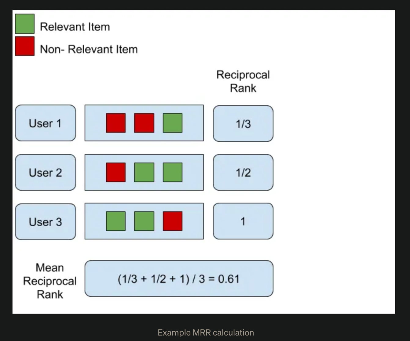
Mean Reciprocal Rank

1
2
3
4
5
6
7
8
9
10
11
12
13
14
15
16
17
18
19
20
21
22
23
24
25
26
27
28
29
30
31
32
33
34
35
def mean_reciprocal_rank(recommended_items_list, relevant_items_list):
if len(recommended_items_list) != len(relevant_items_list):
raise ValueError("The length of recommended_items_list and relevant_items_list must be the same.")

reciprocal_ranks = []

# Iterate through the lists of recommended items and relevant items for each user
for recommended_items, relevant_items in zip(recommended_items_list, relevant_items_list):
# Find the reciprocal rank for each user
for rank, item in enumerate(recommended_items, start=1):
if item in relevant_items:
reciprocal_ranks.append(1 / rank)
break
else:
reciprocal_ranks.append(0)

# Calculate the mean reciprocal rank
mrr = sum(reciprocal_ranks) / len(reciprocal_ranks)
return mrr

# Example usage
recommended_items_list = [
[1, 3, 5, 7, 9], # user 1
[2, 4, 6, 8], # user 2
[11, 12, 13, 14, 15, 16, 17] # user 3
]

relevant_items_list = [
[2, 3, 5, 7, 11], # user 1
[1, 4, 6, 8, 9], # user 2
[16, 17, 18, 19, 20] # user 3
]

mrr = mean_reciprocal_rank(recommended_items_list, relevant_items_list)
print(f"Mean Reciprocal Rank: {mrr:.2f}") # 0.39

Mean Average Precision (MAP)

Similar to MRR, it calculates the average precision for each user and takes the mean across all users. It takes into account both the order and the relevance of recommended items. The larger value is, the better the recommendation quality is.

  • Pros
    • Position-aware: MAP takes into account the position of relevant items in the recommendation list, rewarding systems that rank relevant items higher.
    • Relevance-aware: MAP considers the relevance of items by calculating the average precision for each user, which is the average of the precision scores at each relevant item’s position.
    • Average performance: MAP calculates the mean average precision across all users, providing an overall measure of the recommendation system’s performance.
    • Robustness: MAP is less sensitive to outliers compared to some other metrics, as it calculates the average precision across multiple positions in the recommendation list for each user.
  • Cons
    • Binary relevance assumption, e.g., on a scale from 1 to 5 stars, the evaluation would need first to threshold the ratings to make binary relevancies. One option is to consider only ratings bigger than 4 as relevant. This introduces bias in the evaluation metric because of the manual threshold[4].
    • Lack of personalization
    • Not suitable for all scenarios: MAP is more appropriate for recommendation scenarios where a ranked list of items is provided to users. It may not be suitable for other types of recommendation scenarios, such as collaborative filtering or content-based recommendations that do not involve explicit ranking.
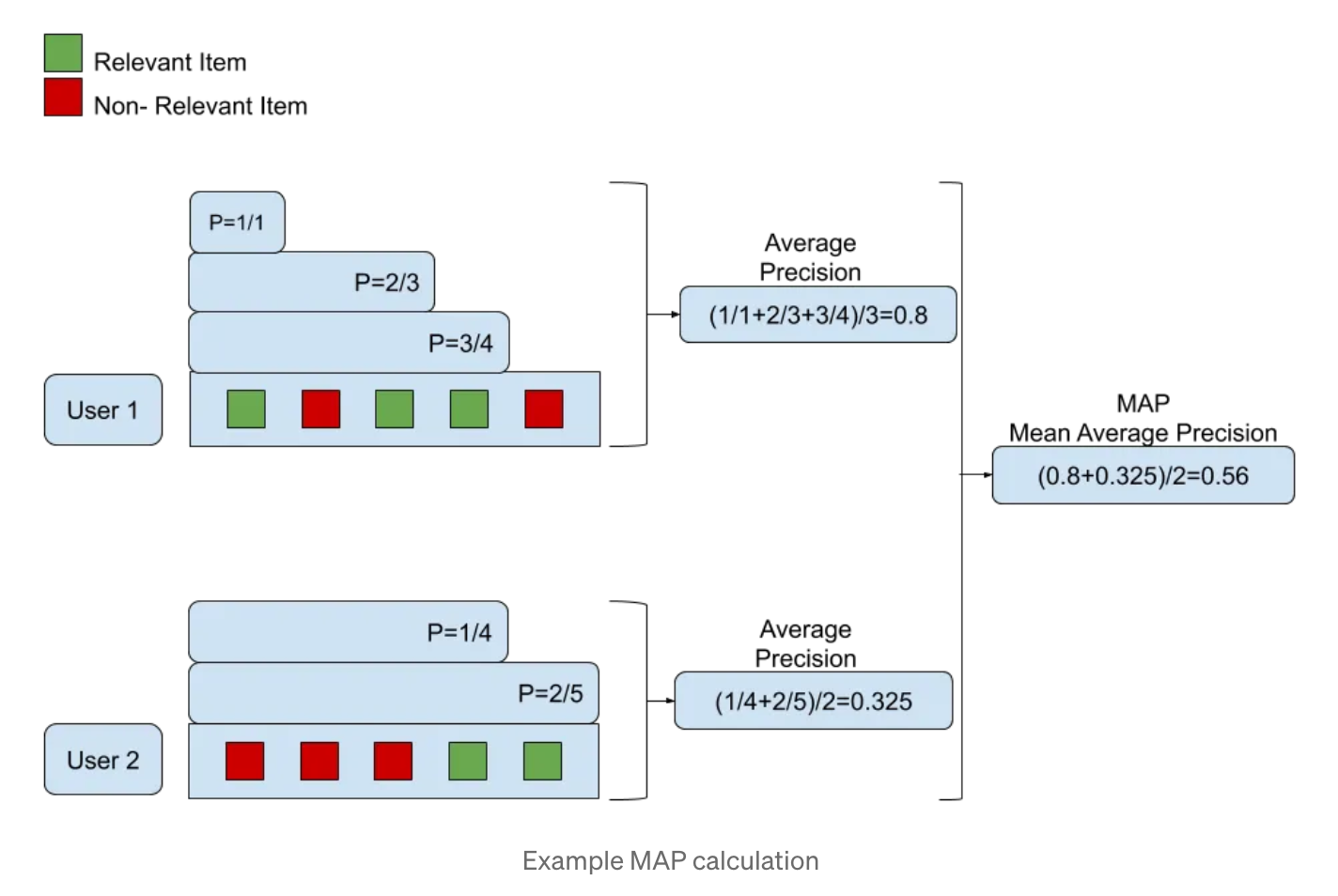
Mean Average Precision

1
2
3
4
5
6
7
8
9
10
11
12
13
14
15
16
17
18
19
20
21
22
23
24
25
26
27
28
29
30
31
32
33
34
35
36
37
38
39
40
41
42
43
def average_precision(recommended_items, relevant_items):
true_positives = 0
sum_precisions = 0

for rank, item in enumerate(recommended_items, start=1):
if item in relevant_items:
true_positives += 1
precision_at_rank = true_positives / rank
sum_precisions += precision_at_rank

return sum_precisions / len(relevant_items) if len(relevant_items) > 0 else 0


def mean_average_precision(recommended_items_list, relevant_items_list):
if len(recommended_items_list) != len(relevant_items_list):
raise ValueError("The length of recommended_items_list and relevant_items_list must be the same.")

average_precisions = []

# Calculate the average precision for each user
for recommended_items, relevant_items in zip(recommended_items_list, relevant_items_list):
ap = average_precision(recommended_items, relevant_items)
average_precisions.append(ap)

# Calculate the mean average precision across all users
map_value = sum(average_precisions) / len(average_precisions)
return round(map_value, 2)

# Example usage
recommended_items_list = [
[1, 3, 5, 7, 9],
[2, 4, 6, 8],
[11, 12, 13, 14, 15, 16, 17]
]

relevant_items_list = [
[2, 3, 5, 7, 11],
[1, 4, 6, 8, 9],
[16, 17, 18, 19, 20]
]

map_value = mean_average_precision(recommended_items_list, relevant_items_list)
print(f"Mean Average Precision: {map_value}") # 0.29

Normalized Discounted Cumulative Gain (nDCG)

Given the fact that most relevant items are more useful than irrelevant items, nDCG evaluates the ranking quality by assigning higher importance to relevant items appearing at the top of the recommendation list. It is normalized to ensure comparability across different users and queries.

  • Cumulative Gains (CG): It sums the items based on its relevancy, hence, the term cumulative. For example, if we score the relevance, most relevant score => 2, somewhat relevant score => 1, least relevant score => 0.

  • Discounted Cumulative Gains (DCG): It penalized the items that appear lower in the list. A relevant item appearing at the end of the list is a result of a bad recommender system and hence that item should be discounted. To do so we divide the relevance score of items with the log of its rank on the list.

  • Normalized Discounted Cumulative Gains (nDCG): nDCG normalized the DCG values of the different number of the items lists. To do so we sort the item list by relevancy and calculate the DCG for that list. This will be the perfect DCG score as items are sorted by their relevancy score. We divide all DCG score of all the list we get by this perfect DCG to get the normalized score for that list.

  • Pros

    • Position-aware: Items that are ranked higher (closer to the top) contribute more to the nDCG score, reflecting the fact that users are more likely to interact with items at the top of the list.
    • Relevance-weighted: nDCG incorporates the relevance of each recommended item, allowing it to differentiate between items with varying degrees of relevance. This makes it suitable for situations where the relevance of items is not binary (e.g., partially relevant, highly relevant) and can be quantified on a continuous scale.
    • Normalized: nDCG is normalized against the ideal ranking, which means it can be compared across different queries or users.
    • Suitable for diverse recommendation scenarios: nDCG is applicable to various recommendation scenarios, including search engine result ranking, collaborative filtering, and content-based recommendation.
    • Intuitive interpretation: nDCG scores range from 0 to 1, with higher values indicating better ranking quality.
  • Cons

    • Lack of personalization
    • Binary relevance assumption: Although nDCG can handle varying degrees of relevance, it is often used with binary relevance judgments in practice.
    • Sensitive to the choice of the ideal ranking: The normalization factor in nDCG is based on the ideal ranking, which can sometimes be subjective or difficult to determine. The choice of the ideal ranking can influence the nDCG score, potentially affecting its consistency and reliability.
1
2
3
4
5
6
7
8
9
10
11
12
13
14
15
16
17
18
19
20
21
22
23
24
25
26
27
28
29
30
31
32
33
34
35
36
37
38
import math
def discounted_cumulative_gain(recommended_items, relevant_items):
dcg = 0
for i, item in enumerate(recommended_items, start=1):
if item in relevant_items:
dcg += 1 / (math.log2(i + 1))
return dcg

def ideal_discounted_cumulative_gain(recommended_items, relevant_items):
sorted_relevant_items = sorted(relevant_items, key=lambda x: recommended_items.index(x) if x in recommended_items else float('inf'))
return discounted_cumulative_gain(sorted_relevant_items, relevant_items)

def normalized_discounted_cumulative_gain(recommended_items, relevant_items):
dcg = discounted_cumulative_gain(recommended_items, relevant_items)
idcg = ideal_discounted_cumulative_gain(recommended_items, relevant_items)

if idcg == 0:
return 0
else:
return round(dcg / idcg, 2)

# Example usage
recommended_items_list = [
[1, 3, 5, 7, 9],
[2, 4, 6, 8],
[11, 12, 13, 14, 15, 16, 17]
]

relevant_items_list = [
[2, 3, 5, 7, 11],
[1, 4, 6, 8, 9],
[16, 17, 18, 19, 20]
]

ndcg_values = [normalized_discounted_cumulative_gain(recommended, relevant)
for recommended, relevant in zip(recommended_items_list, relevant_items_list)]

print(f"nDCG values: {ndcg_values}") # [0.53, 0.53, 0.23]

Spearman Rank Correlation Evaluation [2] [12]

Pearson Correlation [12] [14]

Rank-Biased Precision (RBP) [15]

Expected Reciprocal Rank (ERR) [15]

Coverage and Diversity Metrics

Catalog Coverage

It measures the proportion of items in the catalog that are recommended at least once.

1
2
3
4
5
6
7
8
9
10
11
12
13
14
15
16
17
18
19
20
21
22
def catalog_coverage(recommended_items_list, catalog_items):
# Flatten the list of recommended items and convert it to a set
unique_recommended_items = set(item for sublist in recommended_items_list for item in sublist)

# Calculate the intersection of unique recommended items and catalog items
covered_items = unique_recommended_items.intersection(catalog_items)

# Calculate the catalog coverage
coverage = len(covered_items) / len(catalog_items)
return coverage

# Example usage
recommended_items_list = [
[1, 3, 5, 7, 9], # user 1
[2, 4, 6, 8], # user 2
[11, 12, 13, 14, 15, 16, 17] # user 3
]

catalog_items = set(range(1, 21))

coverage = catalog_coverage(recommended_items_list, catalog_items)
print(f"Catalog Coverage: {coverage}") # 0.8

Prediction Coverage

It measures the proportion of possible user-item pairs for which the recommendation system can make predictions.

1
2
3
4
5
6
7
8
9
10
11
12
13
14
15
16
17
18
19
20
21
22
23
def prediction_coverage(predicted_ratings, total_users, total_items):
# Count the number of user-item pairs for which the recommendation system can make predictions
predicted_pairs = sum(len(ratings) for ratings in predicted_ratings)

# Calculate the total number of possible user-item pairs
total_possible_pairs = total_users * total_items

# Calculate the prediction coverage
coverage = predicted_pairs / total_possible_pairs
return coverage

# Example usage
predicted_ratings = [
{1: 3.5, 3: 4.0, 5: 2.5, 7: 3.0, 9: 4.5}, # user 1, item 1 has the predicted rating of 3.5, item 9 has the predicted rating of 4.5.
{2: 4.5, 4: 3.0, 6: 2.0, 8: 3.5}, # user 2
{11: 3.5, 12: 4.0, 13: 2.5, 14: 3.0, 15: 4.5, 16: 3.5, 17: 2.0} # user 3
]

total_users = 3
total_items = 20

coverage = prediction_coverage(predicted_ratings, total_users, total_items)
print(f"Prediction Coverage: {coverage:.2f}")

Diversity

It helps ensure personalized and engaging experiences for users, supports exploration, reduces filter bubbles, promotes long-tail items, and enhances the robustness of the system.

1
2
3
4
5
6
7
8
9
10
11
12
13
14
15
16
17
18
19
20
21
22
23
24
25
26
27
28
29
30
31
32
33
import numpy as np
from sklearn.metrics.pairwise import cosine_similarity

def diversity(recommended_items_list, item_features):
total_similarity = 0
total_pairs = 0

for recommended_items in recommended_items_list:
# Calculate pairwise cosine similarities for the recommended items
similarities = cosine_similarity([item_features[item] for item in recommended_items])
# Sum the similarities for all item pairs
total_similarity += np.sum(similarities) - np.trace(similarities) # Exclude the diagonal
# Count the total number of item pairs
total_pairs += len(recommended_items) * (len(recommended_items) - 1)

# Calculate the average similarity between item pairs
avg_similarity = total_similarity / total_pairs if total_pairs > 0 else 0
# Calculate the diversity by subtracting the average similarity from 1
diversity = 1 - avg_similarity
return diversity

# Example usage
recommended_items_list = [
[1, 3, 5, 7, 9], # user 1
[2, 4, 6, 8], # user 2
[11, 12, 13, 14, 15, 16, 17] # user 3
]

# Example item features dictionary (using 5-dimension random feature vector)
item_features = {item: np.random.rand(5) for item in range(1, 21)}

diversity_value = diversity(recommended_items_list, item_features)
print(f"Diversity: {diversity_value:.2f}") # 0.23

Serendipity

It measures the degree to which the recommended items are both relevant and unexpected, promoting the discovery of novel and interesting items. A recommendation list with serendipity can introduce users to items they may not have expected to enjoy or find relevant, leading to serendipitous discoveries. This can create a more enjoyable and engaging user experience.

Measuring serendipity is a challenging task as it involves the combination of relevance, surprise, and novelty. Here’s a Python function to calculate a basic version of Serendipity, which measures the degree to which the recommended items are both relevant and unexpected:

1
2
3
4
5
6
7
8
9
10
11
12
13
14
15
16
17
18
19
20
21
22
23
24
25
26
27
28
29
30
31
32
33
34
35
36
37
38
def serendipity(recommended_items_list, relevant_items_list, popular_items, k=10):
serendipity_score = 0
total_users = len(recommended_items_list)

for recommended_items, relevant_items in zip(recommended_items_list, relevant_items_list):
# Select the top-k recommended items
top_k_recommended = recommended_items[:k]

# Find the serendipitous items by removing popular items from relevant items
serendipitous_items = set(relevant_items) - set(popular_items)

# Count the number of serendipitous items in the top-k recommendations
serendipitous_recommendations = len(set(top_k_recommended) & serendipitous_items)

# Calculate the proportion of serendipitous items in the top-k recommendations
serendipity_score += serendipitous_recommendations / k

# Calculate the average serendipity score across all users
avg_serendipity = serendipity_score / total_users
return avg_serendipity

# Example usage
recommended_items_list = [
[1, 3, 5, 7, 9, 2, 4, 6, 8, 11], # user 1
[2, 4, 6, 8, 1, 3, 5, 7, 9, 12], # user 2
[11, 12, 13, 14, 15, 16, 17, 1, 3, 5] # user 3
]

relevant_items_list = [
[2, 3, 5, 7, 11, 13, 15, 17],
[1, 4, 6, 8, 9, 11, 14, 16],
[1, 3, 5, 7, 9, 11, 12, 13, 15, 17]
]

popular_items = [1, 2, 3, 4, 5, 6, 7, 8, 9]

serendipity_value = serendipity(recommended_items_list, relevant_items_list, popular_items)
print(f"Serendipity: {serendipity_value:.2f}") # 0.20

Popularity[2]

Novelty[2]

Hit Ratio (HR)[5]

It is the fraction of users for which the relevant item is included in the recommendation list of length K.

HR=UhitKUall\text{HR} = \frac{|U^K_{hit}|}{|U_{all}|}

|UKhit| is the number of users for which the relevant item is included in the top K recommended items ||Uall| | is the total number of users in the test dataset.

Reference